Digital Oscilloscope: Signal Acquisition, Sampling and Waveform Analysis
Digital Oscilloscope
LABORATORY MEASUREMENT SYSTEMS · TOPIC 04.03 · SIGNAL ACQUISITION
An oscilloscope displays how an electrical signal changes with time. Unlike a digital multimeter, which commonly reports a numerical value processed over a measurement interval, an oscilloscope preserves time-dependent information such as transients, oscillations, switching events, noise and waveform distortion.
Central idea: an oscilloscope does not simply show the signal. It conditions the input, samples it in time, converts the samples into digital values, stores them and reconstructs a visual representation according to the acquisition settings.
1. What does an oscilloscope measure?
The primary measured quantity is voltage as a function of time, (v(t)). From the acquired waveform, the instrument can estimate peak and RMS voltage, period, frequency, rise and fall time, pulse width, duty cycle, phase difference, overshoot, ringing and noise. Some instruments also provide FFT-based spectral analysis.
Most general-purpose oscilloscopes measure voltage. Current is usually inferred using a current probe or a voltage drop across a known shunt resistor. The probe and measurement method must be included in the interpretation.
2. The oscilloscope signal chain
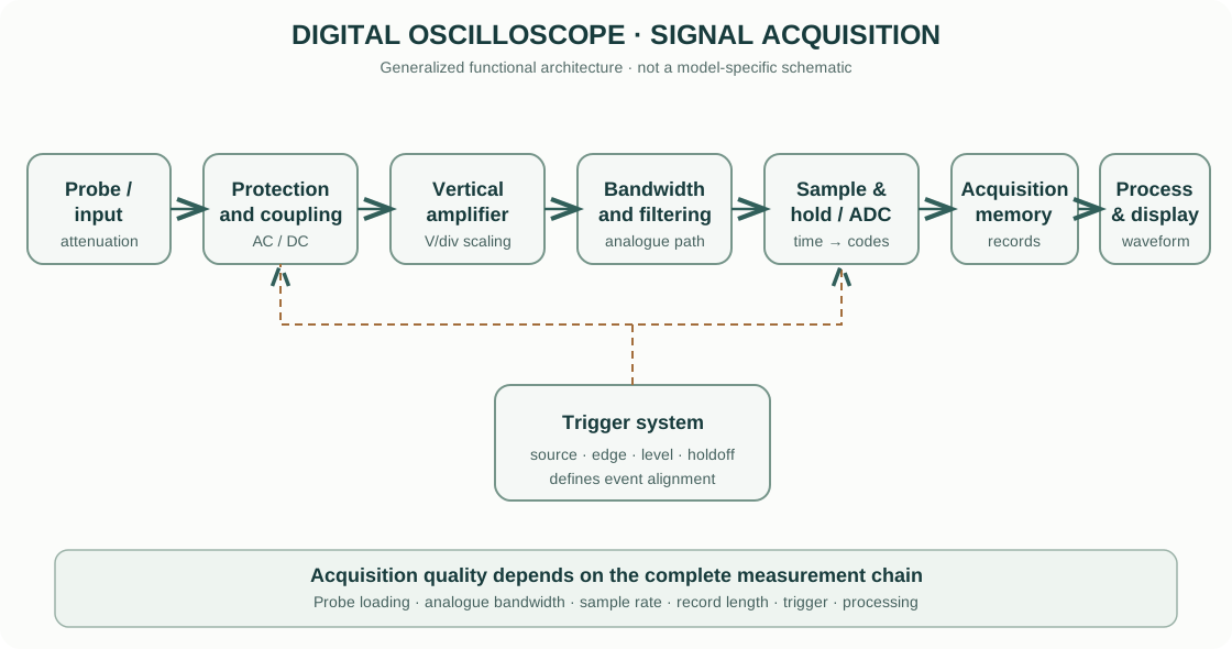
- Probe and input connector: connect the instrument to the circuit while providing a defined attenuation, impedance and grounding arrangement.
- Input protection and coupling: protect the front end within specified limits and select AC coupling, DC coupling or ground reference where available.
- Vertical amplifier / attenuator: scale the signal to fit the ADC input range. The volts-per-division setting determines the displayed vertical scale.
- Bandwidth-limiting path: the analogue front end has a finite frequency response. Some instruments provide selectable bandwidth limits to reduce high-frequency noise.
- Sample-and-hold and ADC: sample the conditioned signal at discrete times and convert each sample into a digital code.
- Acquisition memory: store samples for display and processing. Record length and sample rate determine the time span and time resolution available in a capture.
- Trigger system: identify a defined event, such as a rising edge crossing a threshold, to stabilize the displayed waveform or capture a single event.
- Processing and display: apply interpolation, measurements, math functions and display persistence to render the acquired data.
This is a generalized functional architecture. Actual instruments may use interleaved ADCs, multiple acquisition paths, digital trigger engines and different memory arrangements.
3. Vertical system: volts per division
The vertical system controls how input voltage maps to the screen. If a waveform occupies (N_v) vertical divisions and the selected scale is (S_v) volts per division, its displayed peak-to-peak voltage is approximately:
[ V_{pp}=N_v S_v A_p ]
where (A_p) is the probe attenuation factor when the oscilloscope does not automatically account for it. If a 10× probe is connected but the channel is configured as 1×, the displayed voltage will be wrong by a factor of ten.
Probe attenuation and loading
A passive probe commonly uses a compensated divider. A 10× probe reduces the signal reaching the oscilloscope by approximately a factor of ten and usually presents a higher input resistance to the circuit than a direct 1× connection. Probe capacitance and compensation matter, particularly for fast edges.
The probe is part of the measurement system. Its bandwidth, attenuation, input capacitance, voltage rating and ground-lead inductance can change the observed waveform.
4. Horizontal system: time per division
The horizontal scale sets the time represented by each division. For a waveform spanning (N_t) divisions at (S_t) seconds per division:
[ T_{display}=N_t S_t ]
For a periodic signal, frequency is:
[ f= ]
A wider time window shows more cycles but may reduce the available sample rate or force the instrument to decimate data, depending on acquisition mode and memory depth.
5. Sampling and the Nyquist criterion
A digital oscilloscope samples the analogue input at discrete time intervals. The sample rate (f_s) is the number of samples acquired per second. The sampling interval is:
[ t= ]
For a band-limited signal with maximum frequency (f_{max}), the ideal Nyquist condition requires:
[ f_s>2f_{max} ]
This is a theoretical minimum for perfect reconstruction under ideal band-limiting assumptions. It is not a practical recommendation to set the oscilloscope to only twice the highest frequency of interest. Real waveforms contain harmonics, finite rise times and noise; practical acquisition normally requires substantially more samples per cycle or per edge.
Aliasing
If the sample rate is too low, higher-frequency components can appear as false lower-frequency components. This is aliasing. It can make a waveform look slower, distort its apparent frequency or hide fast events.
Reduce aliasing by using a sample rate appropriate to the highest relevant signal content, checking the analogue bandwidth and bandwidth-limit setting, selecting a suitable acquisition mode, and increasing record length when a long time window and high sample rate are both required.
6. Bandwidth and rise time
Oscilloscope bandwidth is usually specified as the frequency at which the response to a sinusoidal input has fallen by approximately 3 dB from its low-frequency value. At this point the measured amplitude is about 70.7% of the low-frequency amplitude.
A common approximation for the rise time of a single-pole response is:
[ t_r ]
where (BW) is in hertz and (t_r) is in seconds. This approximation is not universal; the relationship depends on the instrument response and measurement definition.
For a signal edge with rise time (t_{r,signal}), the observed rise time is often approximated by:
[ t_{r,meas} ]
This relation is useful for approximately Gaussian responses. If the oscilloscope rise time is comparable to the signal rise time, the instrument significantly affects the result.
7. Triggering: making the waveform stable
The trigger system defines the event at which acquisition or display alignment occurs. A basic edge trigger starts or aligns acquisition when the input crosses a selected voltage threshold in a selected direction.
Important controls include trigger source, slope, level, mode (auto, normal or single, depending on the instrument) and holdoff. Triggering does not improve intrinsic signal-to-noise ratio; it helps capture or display a repeatable event. A poorly selected trigger can produce an unstable display even when the underlying signal is periodic.
8. Acquisition modes and memory
- Sample: stores samples at the acquisition rate.
- Peak detect: retains extrema within acquisition intervals to reveal narrow events, subject to instrument implementation.
- Average: averages repeated acquisitions to reduce uncorrelated noise; it can suppress non-repeatable events.
- High resolution: uses processing or oversampling to improve effective vertical resolution over a reduced bandwidth.
- Segmented memory: stores multiple triggered records while ignoring long intervals between events.
Record length is the number of samples stored per acquisition. For a fixed sample rate, a longer record captures a longer time interval. For a fixed time window, a longer record can preserve a higher sample density.
9. Practical measurement workflow
- Identify the circuit reference, expected voltage, signal frequency and transient content.
- Select a probe with suitable attenuation, bandwidth, voltage rating and input capacitance.
- Check the oscilloscope input rating and the probe’s maximum voltage and category ratings.
- Connect the probe ground only to a point that is safe to reference to the oscilloscope ground. Many bench oscilloscopes have earth-referenced ground clips; connecting them to a live or floating node can create a short circuit.
- Compensate an adjustable passive probe using the instrument’s calibration output, following the probe manual.
- Select DC coupling when the DC level matters; use AC coupling only when intentionally removing the DC component.
- Set volts/division and time/division to show the signal without clipping or excessive empty display.
- Choose a suitable sample rate, record length, bandwidth and acquisition mode.
- Set trigger source, slope and level to obtain a stable capture.
- Use automatic measurements as a starting point, then inspect the waveform and measurement gates manually.
- Save the waveform and settings. Record probe attenuation, bandwidth limit, sample rate, time base, trigger settings and relevant measurement statistics.
10. Common sources of error
| Error source | What happens | How to control it |
|---|---|---|
| Probe loading | Probe resistance/capacitance changes the circuit | Use a suitable low-capacitance or active probe |
| Ground-lead inductance | Creates ringing or overshoot on fast edges | Use a short ground spring or appropriate differential probe |
| Insufficient bandwidth | Attenuates fast edges and high-frequency components | Select adequate bandwidth and probe |
| Low sample rate | Causes aliasing or missed transients | Increase sample rate and verify acquisition mode |
| Incorrect probe factor | Voltage scale is wrong | Match probe attenuation in channel settings |
| Poor trigger setup | Display appears unstable or events are missed | Select correct source, slope, level and mode |
| AC coupling | Removes DC component and affects low-frequency response | Use DC coupling when DC content matters |
| Averaging | Hides non-repeatable events | Use sample or single-shot acquisition for transients |
| Ground reference error | Can short a circuit node or create ground-loop current | Understand earth reference and use rated differential isolation |
11. Commercial oscilloscope examples
These official manufacturer resources are starting points for comparing instrument families. They are not endorsements, and capabilities vary substantially by model.
- Tektronix — Oscilloscopes: general-purpose, mixed-signal and high-performance oscilloscope families, with application notes and manuals.
- Keysight — Oscilloscopes: InfiniiVision and Infiniium families, probes and application resources.
- Rohde & Schwarz — Oscilloscopes: digital oscilloscope product families and technical resources.
- Yokogawa Test & Measurement: waveform measurement instruments and application information.
When comparing models, check analogue bandwidth, maximum real-time sample rate, memory depth, ADC resolution and effective number of bits, channel count, trigger capability, probe ecosystem, input rating, isolation and software options. A headline sample rate alone is not enough to judge measurement performance.
12. Intellectual-property and educational scope
The explanatory text and functional signal-chain diagram on this page are original educational material. The diagram is a generalized conceptual representation, not a reproduction of a manufacturer’s schematic or user manual. Manufacturer names and product links identify their respective products; trademarks, product images, manuals and specifications remain the property of their owners. Use the current documentation for the exact model and probe.
This guide explains general oscilloscope principles. It does not replace the instrument manual, electrical-safety training, probe ratings, calibration procedure or laboratory risk assessment.