Digital Multimeter (DMM): Operating Principles and Measurement Practice
Digital Multimeter (DMM)
LABORATORY MEASUREMENT SYSTEMS · TOPIC 04.01 · FOUNDATIONAL LEVEL
A digital multimeter (DMM) converts an electrical quantity at its input terminals into a numerical result. It can measure several different quantities, but it does not use one identical measurement method for all of them. Voltage, current and resistance require different input circuits, protection arrangements and conversion procedures.
Central idea: the display is the final stage of a measurement chain. A trustworthy reading depends on the input connection, range, analogue conditioning, analogue-to-digital conversion, timing, calibration and the electrical behaviour of the specimen.
1. What does a DMM measure?
| Mode | Quantity | Basic principle |
|---|---|---|
| DC voltage | Potential difference, V | High-impedance differential measurement |
| AC voltage | Time-varying potential difference | AC coupling/conditioning and RMS estimation |
| DC current | Charge flow per unit time, A | Voltage drop across an internal shunt or current-sense element |
| AC current | Alternating current, A | Current-to-voltage conversion followed by AC processing |
| Resistance | Opposition to current, Ω | Apply a known test current or voltage and measure the response |
| Continuity / diode | Electrical path or junction response | Apply a limited test stimulus and evaluate the measured voltage |
| Capacitance / frequency / temperature | Model-dependent derived quantity | Dedicated excitation and signal-processing functions |
Not every DMM supports every mode. The measurement range, accuracy, bandwidth, input protection and test stimulus are model-dependent.
2. The internal measurement chain
The following original functional diagram explains a common DMM architecture. It is not a circuit schematic for a particular commercial model; manufacturers differ in their analogue front ends, ADC topology, protection and internal switching.
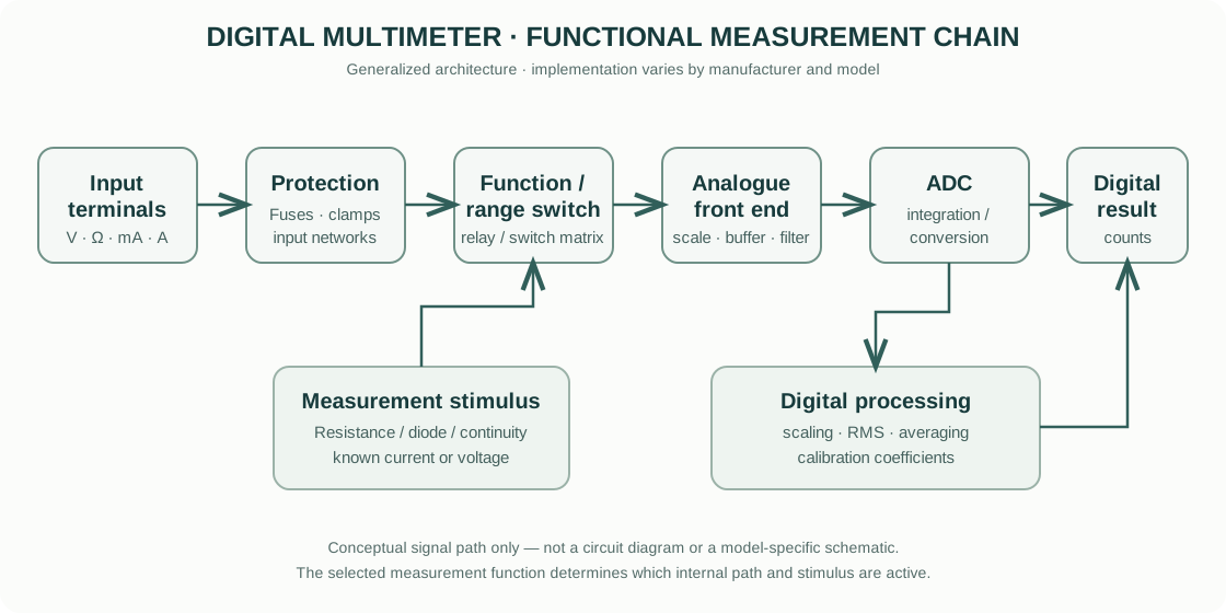
- Input terminals and protection: the selected terminals connect the instrument to the circuit. Fuses, transient protection and input networks reduce the risk of damage under specified conditions.
- Function and range switching: internal relays or semiconductor switches route the input through the appropriate measurement path. The selected range determines scaling and often affects resolution, noise and accuracy.
- Analogue front end: attenuators scale voltage; current ranges use a shunt; resistance mode applies a known test stimulus. Buffer amplifiers and filters condition the signal.
- Analogue-to-digital conversion (ADC): the conditioned analogue signal is converted into a digital representation. Integrating ADCs, including dual-slope architectures, are common in precision DMMs because of their noise-rejection characteristics; faster instruments may use different conversion architectures.
- Digital processing: the instrument applies scaling, linearization, filtering, averaging, AC calculations and calibration coefficients as appropriate to the selected function.
- Display and communication: the result, units, range and status are displayed or transferred through an interface. A displayed number does not by itself communicate the full uncertainty.
3. How each measurement mode works
3.1 DC voltage
A voltmeter is connected in parallel with the element whose potential difference is being measured. Ideally, the meter draws no current. A real DMM has a finite input resistance, commonly around 10 MΩ on many voltage ranges, although this is not universal.
The input resistance forms a divider with the source resistance:
[ V_{meas}=V_s ]
where (V_s) is the source voltage, (R_s) is source resistance and (R_{in}) is the DMM input resistance.
Example: a 10 V source with 1 MΩ source resistance connected to a 10 MΩ input gives approximately 9.09 V. The difference is loading error, not necessarily a defective meter.
3.2 DC current
An ammeter is connected in series so that the circuit current passes through its current-measurement path. A common architecture measures the voltage across a known low-value shunt resistor:
[ I= ]
The shunt produces a burden voltage that can alter the circuit being measured. A lower shunt resistance reduces burden voltage but makes the sensed voltage smaller and can increase the difficulty of resolving low currents.
Critical connection rule: never place a DMM configured for current measurement directly across a voltage source. The low-resistance current path can create a short circuit and may blow the fuse or damage the instrument.
3.3 Resistance
A DMM cannot determine resistance by simply observing an unpowered component. It applies a known test current (or a controlled test voltage), measures the resulting voltage (or current), and calculates:
[ R= ]
The component should normally be isolated from external power. Parallel circuit paths can produce a result lower than the component’s actual resistance. Semiconductor junctions and capacitors can also affect readings.
For low resistance, lead and contact resistance become significant. A four-wire (Kelvin) method uses one pair of leads to force current and a separate high-impedance pair to sense voltage:
[ R_x= ]
This reduces the contribution of lead resistance, but it does not eliminate errors caused by poor contacts, thermal EMFs, specimen heating or unsuitable test current.
3.4 AC voltage and true RMS
For a periodic voltage, the RMS value is:
[ V_{RMS}= ]
For a pure sine wave, (V_{RMS}=V_{peak}/). This shortcut is not generally valid for distorted or non-sinusoidal waveforms. A true-RMS DMM estimates RMS over its supported bandwidth and crest-factor limits. Average-responding meters calibrated to display the RMS value of a sine wave can give incorrect results for non-sinusoidal signals.
4. Resolution, accuracy and sensitivity are not interchangeable
- Resolution: the smallest change in input that can produce a change in the displayed count under a stated range and configuration.
- Accuracy specification: the manufacturer’s stated measurement-error limit under specified conditions, often expressed as a percentage of reading plus a percentage of range or counts.
- Repeatability: the closeness of repeated results under the same conditions.
- Sensitivity: how much the indicated output changes for a change in input; in a digital display this is related to the measurement range and quantization.
A 6½-digit display does not mean that every reading is accurate to one part in ten million. Accuracy depends on the complete specification, calibration interval, temperature coefficient, range, integration time and measurement conditions.
A common specification format is:
[ ( a%;of;reading+b%;of;range ) ]
The exact manufacturer convention must be checked in the datasheet. Do not compare two instruments using digit count alone.
5. Integration time and noise rejection
Many precision DMMs integrate the input over a defined time. Integration time is often specified in power-line cycles (NPLC). An integration window synchronized to an integer number of mains cycles can reject much of the corresponding line-frequency interference.
Longer integration generally improves rejection of low-frequency noise and stability, but reduces reading speed. Shorter integration enables faster acquisition but may increase noise and uncertainty. The appropriate setting depends on whether the experiment prioritizes stable precision readings or time-resolved changes.
6. Practical measurement workflow
- Identify the quantity and expected magnitude before connecting the meter.
- Inspect leads, insulation, probes, fuses and terminal labels.
- Select the correct function and input terminals. Start with a range that safely covers the expected value.
- For voltage, connect in parallel. For current, open the circuit and connect in series. For resistance, isolate the specimen and remove external power.
- Allow the instrument and specimen to stabilize where thermal EMFs or drift may matter.
- Record function, range, integration time, AC bandwidth (if relevant), instrument model and calibration status.
- Repeat the measurement and check stability. For low-level signals, reverse polarity or use a suitable offset-correction procedure when justified.
- Report the value with units, relevant settings and uncertainty—not just the displayed digits.
7. Common sources of error
| Error source | Mechanism | Practical response |
|---|---|---|
| Loading | Finite input resistance changes circuit voltage | Use a higher-input-impedance instrument or buffer |
| Lead/contact resistance | Adds series resistance to low-ohm measurements | Use four-wire sensing and clean, stable contacts |
| Thermal EMF | Dissimilar-metal junctions generate small thermoelectric voltages | Use suitable copper connections, thermal stability and reversal |
| Electrical noise | EMI, ground loops and mains pickup enter the input | Short leads, shielding, grounding discipline and suitable integration |
| Burden voltage | Current shunt changes the measured circuit | Select an appropriate range or use a low-burden method |
| Range / overload | Incorrect range or transient exceeds limits | Check expected values, ratings and protection |
| Drift / self-heating | Instrument or specimen changes during measurement | Reduce test power, stabilize and repeat |
8. Calibration and verification
Calibration compares the instrument response with traceable standards and documents the result and uncertainty. Verification is a check that the instrument meets a stated requirement; it is not automatically equivalent to a full calibration.
For critical work, use suitable voltage, resistance or current standards and follow the manufacturer’s procedure. Check the calibration certificate, due date, environmental conditions and uncertainty at the range being used. A self-test or zero function does not establish traceability for every range.
9. Commercial instrument examples
These links point to official manufacturer product-family pages. They are examples for learning about available architectures and specifications, not endorsements or a claim that one model is universally best.
- Keysight — Digital Multimeters: handheld, benchtop and modular DMM families, including different resolution and performance classes.
- Tektronix / Keithley — Benchtop Digital Multimeters: instrumentation and precision DMM families, including models with digitizing and data-analysis features.
- ADC Corporation — Digital Multimeters: Japanese manufacturer examples spanning precision bench DMMs and system-calibration instruments.
- Yokogawa Test & Measurement: Japanese measurement-instrument manufacturer and product information.
Always download the datasheet and user manual for the exact model. Check input impedance, current burden voltage, measurement bandwidth, accuracy equation, integration-time options, terminal ratings, fuse type and calibration conditions.
10. Scope and intellectual-property note
The explanatory text and functional diagram on this page are original educational material prepared for this library. The diagram is a generalized conceptual representation and is not copied from a manufacturer manual. Manufacturer names and product-family links are used only to identify their respective products; their trademarks, specifications, manuals and product images remain the property of their owners. Consult the linked manufacturer’s current documentation for authoritative model-specific limits.
Further reading
- Keysight digital multimeter product information
- Keithley benchtop DMM product information
- ADC Corporation DMM product information
This guide explains general measurement principles. It is not a substitute for the instrument manual, electrical-safety training, calibration procedures or laboratory risk assessment.