Thermoelectric Measurement Systems: Seebeck Coefficient, Resistivity and Thermal Conductivity

A practical guide to thermoelectric property measurement, temperature-gradient control, voltage sensing, four-probe resistivity, laser-flash diffusivity and ZT uncertainty.

Thermoelectric Measurement Systems

ELECTROCHEMICAL & TRANSPORT MEASUREMENTS · TOPIC 02.04 · THERMOELECTRIC PROPERTIES

Thermoelectric characterization combines several measurements that are often performed by different modules or instruments. The Seebeck coefficient, electrical resistivity and thermal conductivity are not necessarily measured simultaneously, and their results must be combined only when specimen state, temperature and geometry are compatible.

1. The properties and their roles

The principal quantities are:

• Seebeck coefficient (S), in V K(^{-1});
• electrical conductivity (), in S m(^{-1});
• thermal conductivity (), in W m(^{-1}) K(^{-1});
• dimensionless figure of merit (ZT).

The power factor is:

[ PF=S^2 ]

The dimensionless figure of merit is:

[ ZT= ]

A high Seebeck coefficient alone does not guarantee a high ZT. Electrical and thermal transport must be considered together.

2. Seebeck coefficient measurement

A temperature difference is established across a specimen. The open-circuit thermovoltage is measured using voltage probes or thermocouples connected to a high-input-impedance measurement channel.

Original conceptual diagram of thermoelectric Seebeck measurement

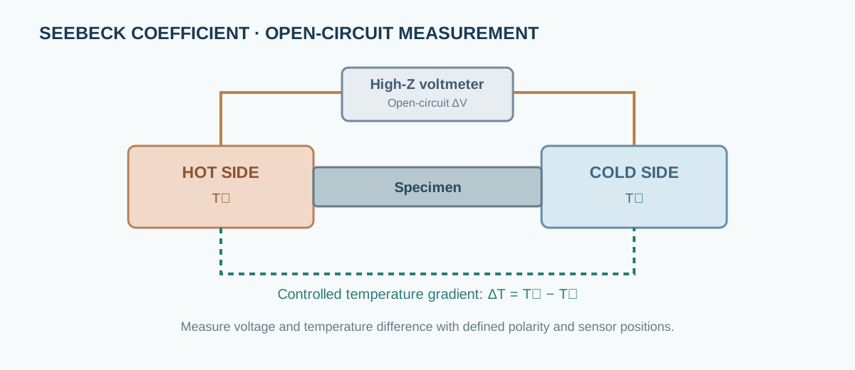
For a small temperature interval where the response is approximately linear:

[ S=- ]

The sign depends on the defined voltage polarity and temperature-gradient direction. Some instruments report the opposite sign convention. Record the wiring convention and confirm it with a reference material.

Use several temperature differences and fit (V) against (T). A single-point ratio is sensitive to offset voltage, parasitic thermoelectric EMFs and temperature-sensor placement.

Important practical details

• Ensure the specimen is clamped reproducibly without excessive contact resistance or thermal shunting.
• Place temperature sensors close to the specimen ends and document their positions.
• Use low-thermal-EMF wiring and stable electrical contacts.
• Allow thermal equilibrium at each setpoint.
• Reverse the gradient when practical to separate odd-in-gradient response from voltage offsets.
• Confirm linearity and repeatability over the chosen temperature interval.

3. Electrical resistivity and conductivity

Electrical resistance is commonly measured with a four-terminal configuration to reduce lead and contact contributions. For a uniform bar of length (L) and cross-sectional area (A):

[ =R,= ]

The current direction, voltage-contact spacing and specimen cross-section must be defined. For temperature-dependent measurements, account for thermal expansion if it is significant relative to the required uncertainty.

A measurement made with two probes can be dominated by contact resistance, especially for semiconducting ceramics or high-resistance specimens.

4. Thermal conductivity: laser flash and related methods

Laser-flash analysis measures thermal diffusivity (), not thermal conductivity directly. A short energy pulse heats one face of a specimen and the temperature rise on the opposite face is monitored. Thermal conductivity is then calculated using:

[ =_m C_p ]

where (_m) is mass density and (C_p) is specific heat capacity. Each quantity must correspond to the same relevant temperature and material state.

Original conceptual diagram of laser-flash thermal diffusivity measurement

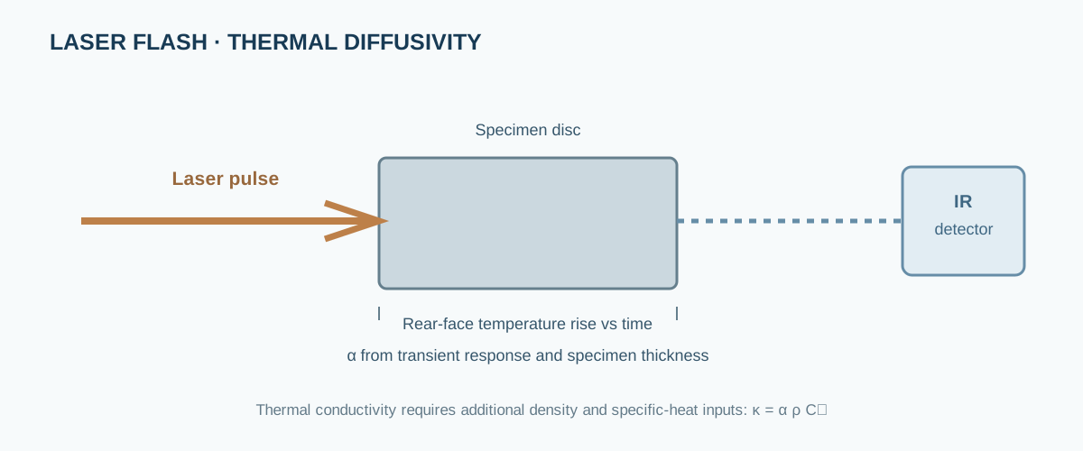
Coating emissivity, sample thickness, heat losses, pulse shape, detector response, porosity and heat-capacity determination can influence the result. The laser-flash instrument does not independently provide all inputs needed for ().

Other methods, including steady-state and comparative techniques, use different physical models and have different contact and boundary-condition requirements. Do not mix diffusivity or conductivity values from different methods without evaluating compatibility.

5. A defensible measurement workflow

1. Prepare specimens with suitable geometry, parallel faces and documented density.
2. Measure dimensions and mass using calibrated instruments.
3. Check thermocouple calibration, polarity and placement.
4. Verify voltage measurement offsets and electrical-contact stability.
5. Establish a controlled temperature gradient and wait for steady state.
6. Record voltage and temperature difference at multiple gradient values.
7. Measure electrical resistance using a suitable four-terminal arrangement.
8. Measure thermal diffusivity and specific heat using validated methods.
9. Repeat measurements and check heating/cooling consistency.
10. Calculate (S), (), (), PF and ZT with propagated uncertainty.

6. Common errors and interpretation limits

Source	Effect	Control
Thermocouple position	Incorrect local (T)	Define sensor spacing and placement
Parasitic thermal EMF	Voltage offset	Low-thermal-EMF leads, gradient reversal
Thermal contact resistance	Temperature drop at interfaces	Reproducible clamping and contact assessment
Electrical contact resistance	Biased resistivity	Four-terminal measurement
Specimen inhomogeneity	Position-dependent properties	Replicate specimens and mapped measurements
Density uncertainty	Direct contribution to calculated ()	State density method and porosity
Temperature mismatch	Invalid combined ZT	Use compatible temperature points and specimen state

7. Uncertainty in ZT

For independent uncertainties, a first-order relative uncertainty estimate is:

[ ()^2 (2)^2+ ()^2+ ()^2+ ()^2 ]

This approximation assumes independent inputs. Correlated uncertainties require covariance terms. Because (S) is squared, its relative uncertainty contributes with a factor of two in this first-order expression.

Do not report excessive significant figures when specimen dimensions, density, thermal contact or temperature gradients dominate the uncertainty.

8. Reporting checklist

Report specimen composition and processing history; geometry and density; measurement direction; temperature range; thermocouple type and placement; voltage polarity convention; gradient values and fitting method; electrical contact configuration; thermal-diffusivity method; specific-heat source or measurement; equations and correction models; replicate count; and uncertainty.

9. Manufacturers and technical documentation

• ULVAC-RIKO — thermoelectric and thermal-property measurement systems.
• ADVANCE RIKO — thermoelectric property measurement equipment.
• NETZSCH — thermal analysis and laser-flash systems.
• Linseis — thermal diffusivity and thermoelectric measurement systems.

Instrument configurations and calculation conventions differ. Consult the exact model documentation and report which module measured each property.