How to Calculate and Measure Thermal Conductivity: Laser Flash, Heat Capacity, and Practical Methods

A practical guide to thermal conductivity in solids and ceramics: Fourier’s law, thermal diffusivity, density, specific heat capacity, laser flash analysis, steady-state methods, Hot Disk, 3-omega and thin-film techniques.

EXPERIMENTAL METHODS · PRACTICAL GUIDE

How to Calculate and Measure Thermal Conductivity: Laser Flash, Heat Capacity, and Practical Methods

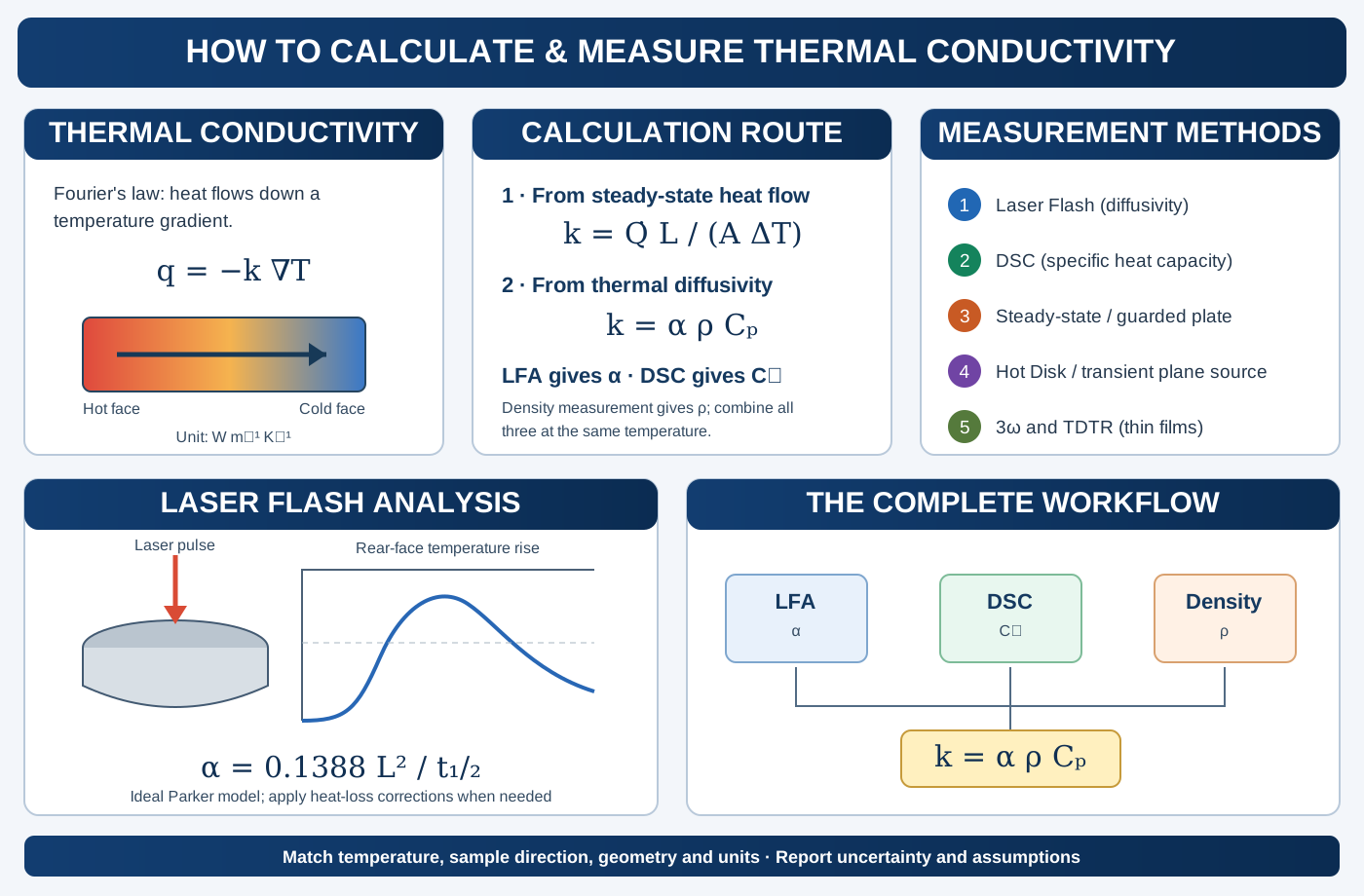
Thermal conductivity is a key property in ceramics, thermoelectric materials, functional oxides, thermal barrier coatings, electronic packaging and energy-conversion devices. It quantifies how readily heat flows through a material in response to a temperature gradient. However, thermal conductivity is not measured by one universal experiment. Some techniques measure conductivity directly under steady-state conditions, whereas others measure thermal diffusivity and require additional measurements of density and specific heat capacity.

This distinction is particularly important when using laser flash analysis (LFA): the laser flash experiment provides thermal diffusivity, not thermal conductivity by itself. The conductivity is then calculated using:

\[ \boxed{k=\alpha\rho C_p} \]

This article explains the physical meaning of each quantity, the main measurement methods, the equations used to calculate thermal conductivity, and the experimental details that matter when measuring ceramic pellets and other solid materials.

Overview of thermal conductivity measurement routes and the relationship between laser-flash diffusivity, DSC heat capacity and density.

1. What is thermal conductivity?

Thermal conductivity, represented by \(k\) or sometimes \(\lambda\), describes the ability of a material to conduct heat. In an isotropic material, Fourier’s law is:

\[ \boxed{\mathbf{q}=-k\nabla T} \]

For one-dimensional heat flow through a flat specimen:

\[ q''=-k\frac{dT}{dx} \]

where \(q''\) is heat flux in W m\(^{-2}\), \(k\) is thermal conductivity in W m\(^{-1}\) K\(^{-1}\), and \(dT/dx\) is the temperature gradient in K m\(^{-1}\). The minus sign indicates that heat flows from higher to lower temperature.

For a homogeneous slab of thickness \(L\), cross-sectional area \(A\), and a steady temperature difference \(\Delta T\):

\[ \boxed{k=\frac{\dot Q L}{A\Delta T}} \]

where \(\dot Q\) is the heat-transfer rate in watts. This equation is the basis of many steady-state measurements. It assumes one-dimensional heat flow, negligible heat loss from the sides, known geometry, and a steady temperature field.

Figure 1. One-dimensional steady-state heat flow through a specimen. The hot and cold faces establish the temperature difference across the sample.

Thermal conductivity versus thermal diffusivity

These quantities are related but not interchangeable:

Property	Symbol	Meaning	SI unit
Thermal conductivity	\(k\)	Ability to conduct heat	W m\(^{-1}\) K\(^{-1}\)
Thermal diffusivity	\(\alpha\)	Rate at which a temperature disturbance spreads	m² s\(^{-1}\)
Density	\(\rho\)	Mass per unit volume	kg m\(^{-3}\)
Specific heat capacity	\(C_p\)	Heat required to raise unit mass by one kelvin at constant pressure	J kg\(^{-1}\) K\(^{-1}\)
Volumetric heat capacity	\(\rho C_p\)	Heat-storage capacity per unit volume	J m\(^{-3}\) K\(^{-1}\)

The relationship is:

\[ \boxed{\alpha=\frac{k}{\rho C_p}} \qquad\Longleftrightarrow\qquad \boxed{k=\alpha\rho C_p} \]

A material can have high thermal diffusivity because it conducts heat efficiently, because it stores relatively little heat per unit volume, or both. Therefore, diffusivity alone does not determine conductivity.

2. The three measurements needed for the LFA calculation

When conductivity is calculated from thermal diffusivity, three independent quantities are required:

1. Thermal diffusivity, \(\alpha\), commonly measured by laser flash analysis.
2. Density, \(\rho\), measured from mass and volume or by an appropriate density method.
3. Specific heat capacity, \(C_p\), commonly measured by differential scanning calorimetry (DSC) or another validated calorimetric method.

The final calculation is:

\[ k=\alpha\times\rho\times C_p \]

Important clarification about DSC: differential scanning calorimetry measures heat flow and is used to determine specific heat capacity. A conventional DSC measurement does not directly provide thermal conductivity. In the LFA workflow, DSC supplies \(C_p\), which is combined with diffusivity and density to calculate \(k\).

3. Laser Flash Analysis (LFA): measuring thermal diffusivity

Laser flash analysis is a transient technique widely used for solid materials, including ceramics, metals, glasses, composites and thermoelectric materials. A short energy pulse heats one face of a thin, usually disk-shaped specimen. An infrared detector records the temperature rise on the opposite face as a function of time.

The characteristic time for the rear face to reach half of its maximum temperature rise is used to calculate thermal diffusivity.

Figure 2. Principle of laser flash analysis: a short pulse heats the front face, while the detector records the transient temperature rise at the rear face.

Parker equation

For an ideal, adiabatic, homogeneous slab with an instantaneous, spatially uniform energy pulse and negligible heat loss, the Parker model gives:

\[ \boxed{\alpha=0.1388\frac{L^2}{t_{1/2}}} \]

where:

• \(L\) is specimen thickness in metres.
• \(t_{1/2}\) is the time required for the rear-face temperature rise to reach half of its maximum value, in seconds.
• \(\alpha\) is thermal diffusivity in m² s\(^{-1}\).

The numerical coefficient 0.1388 belongs to the ideal Parker solution. Real measurements may require corrections for heat loss, finite pulse duration, non-uniform heating, detector response and radiative effects. Modern LFA instruments commonly apply validated analysis models such as Cowan or Cape–Lehman corrections when appropriate.

Worked LFA calculation

Suppose a ceramic disk has:

• Thickness, \(L=2.00\) mm = \(2.00\times10^{-3}\) m.
• Half-rise time, \(t_{1/2}=0.80\) s.

Then:

\[ \alpha=0.1388\frac{(2.00\times10^{-3})^2}{0.80} \]

\[ \boxed{\alpha=6.94\times10^{-7}\;\mathrm{m^2\,s^{-1}}} \]

This is thermal diffusivity, not conductivity. Density and specific heat capacity are still needed.

Practical LFA workflow

1. Prepare a flat, parallel-sided specimen with a thickness appropriate for the instrument and material diffusivity.
2. Measure thickness accurately at several positions; use a representative value and document nonuniformity.
3. Apply a suitable surface coating when required to improve laser absorption and infrared emissivity. The coating must be thin and must not introduce a significant thermal barrier.
4. Measure at the target temperature after thermal stabilization.
5. Record the rear-face temperature-time curve and inspect pulse quality, baseline stability and signal shape.
6. Fit the curve using an appropriate heat-loss model rather than automatically applying the ideal Parker equation to every sample.
7. Repeat shots and, where appropriate, repeat on multiple specimens.

Common LFA limitations: porous or cracked specimens, nonparallel surfaces, poor coating, pulse nonuniformity, large heat losses, anisotropy and temperature gradients can affect the measured diffusivity. For anisotropic materials, the measured direction must be clearly identified.

4. Measuring specific heat capacity: DSC and related methods

Specific heat capacity is a required input to calculate conductivity from diffusivity. Differential scanning calorimetry measures the difference in heat flow between a sample and a reference as temperature changes under a controlled program.

For a calibrated DSC, the heat-flow signal can be related to specific heat capacity. In a simplified calibration-based expression:

\[ C_p(T)=\frac{\dot Q_{sample}(T)-\dot Q_{baseline}(T)} {m\,\beta} \]

where \(\dot Q\) is the relevant heat-flow signal, \(m\) is sample mass and \(\beta=dT/dt\) is the heating rate. The exact instrument equation and calibration procedure depend on the DSC configuration and whether heat-flow or power-compensation DSC is used.

A common practical approach is to measure a baseline, a reference material with known heat capacity (often sapphire), and the sample under matched conditions. The instrument software or validated calibration calculation determines \(C_p(T)\).

DSC measurement considerations

• Use a representative, accurately weighed sample and a suitable pan.
• Calibrate temperature and heat-flow response according to the instrument procedure.
• Measure a reference material with known heat capacity under the same conditions.
• Use matching pans, purge gas, heating rate and measurement conditions for reference and sample.
• Check for mass loss, oxidation, dehydration, phase transitions or other thermal events that can distort the baseline.
• Report whether \(C_p\) is measured at constant pressure and give its temperature dependence when relevant.

Other methods for heat capacity include adiabatic calorimetry and drop calorimetry, depending on the temperature range, sample form and accuracy required.

Do not confuse heat capacity with thermal conductivity: DSC supplies \(C_p\); it does not replace LFA or a direct conductivity measurement.

5. Measuring density for the conductivity calculation

Density is often measured from sample mass and volume:

\[ \boxed{\rho=\frac{m}{V}} \]

For a cylindrical pellet:

\[ V=\pi\left(\frac{D}{2}\right)^2L \]

where \(D\) is diameter and \(L\) is thickness. For porous ceramics, distinguish between bulk density and theoretical crystallographic density. The appropriate density for a macroscopic thermal-conductivity calculation is generally the specimen’s bulk density, because porosity affects the effective heat transport.

For open or closed porosity, Archimedes’ method may be preferable to geometric volume, provided the liquid, saturation and weighing procedure are appropriate for the specimen. State the density method and whether the reported value includes porosity.

6. Combining LFA, DSC and density: full conductivity example

Consider a ceramic sample with the following measured properties at the same temperature:

Quantity	Measured value
Thermal diffusivity, \(\alpha\)	\(6.94\times10^{-7}\) m² s\(^{-1}\)
Bulk density, \(\rho\)	5,000 kg m\(^{-3}\)
Specific heat capacity, \(C_p\)	500 J kg\(^{-1}\) K\(^{-1}\)

Calculate:

\[ k=\alpha\rho C_p \]

\[ k=(6.94\times10^{-7})(5000)(500) \]

\[ \boxed{k=1.735\;\mathrm{W\,m^{-1}\,K^{-1}}} \]

The result is valid only if the three input properties refer to compatible temperatures, material states and measurement directions. For a temperature-dependent study, measure or obtain \(\alpha(T)\), \(\rho(T)\) and \(C_p(T)\) and calculate:

\[ k(T)=\alpha(T)\rho(T)C_p(T) \]

If density is approximated as constant, state that assumption. Thermal expansion can make density temperature-dependent.

7. Other thermal conductivity measurement techniques

LFA is not the only available method. The correct technique depends on the sample geometry, thermal conductivity range, temperature, anisotropy and whether the measurement is transient or steady-state.

7.1 Steady-state method

In a steady-state experiment, a known heat flow passes through a specimen while the temperature difference across a known length is measured. For one-dimensional conduction:

\[ \boxed{k=\frac{\dot QL}{A\Delta T}} \]

Figure 3. Conceptual steady-state arrangement with a hot boundary, cold boundary and specimen between them.

Advantages: conceptually direct and useful for low-to-moderate conductivity materials and insulation.

Limitations: long equilibration times, edge heat losses, contact thermal resistance and the need for carefully guarded one-dimensional heat flow. A guarded hot plate or heat-flow-meter apparatus is often used for standardized measurements of insulating materials.

7.2 Hot Disk / Transient Plane Source (TPS)

The transient plane source method uses a thin sensor, typically a double-spiral metal element, placed between or in contact with specimens. The sensor acts as both a heat source and a temperature-resistance thermometer. The time-dependent temperature response is fitted to a heat-transfer model to obtain thermal conductivity and thermal diffusivity (and, under suitable conditions, volumetric heat capacity).

The method can be convenient for bulk solids, powders, anisotropic materials and some liquids, depending on sensor type and sample configuration.

Important controls: sensor size, sample dimensions, contact pressure, surface flatness, test duration and the validity of the assumed heat-flow geometry. The sample must be sufficiently large relative to the thermal penetration depth during the measurement.

7.3 The 3-omega method

The 3-omega technique is commonly used for thin films, multilayers and bulk materials with suitable geometries. An AC current at angular frequency \(\omega\) passes through a metal line heater. Joule heating contains a component at \(2\omega\), which produces a temperature oscillation. Since the heater resistance changes with temperature, the voltage contains a measurable component at \(3\omega\).

The thermal response is extracted by analyzing the amplitude and phase of the third-harmonic voltage as a function of frequency. The conductivity is obtained by fitting an appropriate heat-diffusion model for the heater, substrate, film and interfaces.

There is no single universal \(k=...\) expression for all 3-omega geometries. The model depends on heater width, film thickness, substrate properties, frequency range, thermal penetration depth and interfacial thermal resistance.

7.4 Thermoreflectance and TDTR

Time-domain thermoreflectance (TDTR) uses a modulated pump laser to heat a metal transducer and a delayed probe laser to monitor changes in reflectivity related to surface temperature. By fitting the delay-dependent signal to a multilayer heat-flow model, TDTR can determine thin-film thermal conductivity and interfacial thermal conductance.

It is especially useful for thin films and interfaces where conventional bulk methods are difficult. Accurate results require a suitable transducer layer, optical calibration, known layer thicknesses and a physically justified multilayer model.

7.5 Comparative methods and heat-flow meters

Comparative techniques determine the unknown conductivity relative to a reference material with known conductivity under similar heat-flow conditions. Heat-flow-meter methods measure heat flux through a specimen under a controlled temperature difference and are widely used for insulation and building materials.

These methods require careful calibration, controlled contact conditions and correction for heat losses. Their suitability depends on the sample’s conductivity range and the relevant testing standard.

8. Which method should you choose?

Sample / objective	Suitable method to consider	Main output
Dense ceramic disk or bulk solid	Laser flash + DSC + density	\(\alpha\), then calculated \(k\)
Low-conductivity insulation	Guarded hot plate or heat-flow meter	Direct steady-state \(k\)
Bulk solid, convenient transient test	Hot Disk / TPS	Model-derived \(k\) and diffusivity
Thin film or multilayer	3-omega or TDTR	Model-derived film/interface properties
Heat capacity only	DSC or calorimetry	\(C_p\)
Comparative testing against a standard	Comparative steady-state method	Relative / calibrated \(k\)

For a typical dense ceramic pellet, LFA combined with DSC and density measurement is a widely used route. If the material is highly anisotropic, layered, porous or has very low thermal conductivity, method selection and geometry corrections become particularly important.

9. Thermal conductivity in ceramics and thermoelectric materials

In crystalline solids, heat can be carried by lattice vibrations (phonons), electrons and, in some materials, other excitations. A useful conceptual decomposition is:

\[ k_{total}=k_{lattice}+k_{electronic}+k_{other} \]

For many electrically insulating oxide ceramics, the lattice contribution dominates. In electrically conducting materials, the electronic contribution can be estimated using the Wiedemann–Franz relation:

\[ k_e=L\sigma T \]

where \(L\) is the Lorenz number, \(\sigma\) is electrical conductivity and \(T\) is absolute temperature. The Lorenz number depends on the carrier statistics and scattering mechanism; using the metallic Sommerfeld value indiscriminately can produce inaccurate estimates in semiconductors and strongly correlated materials.

The lattice contribution may then be estimated as:

\[ k_{lattice}=k_{total}-k_e \]

This subtraction is only as reliable as the conductivity, Lorenz-number model and total thermal-conductivity measurements. Propagate uncertainty and state the assumed Lorenz number.

10. Experimental errors and quality checks

Error source	Effect on result	Control
Incorrect thickness	LFA diffusivity error scales with thickness squared	Measure at multiple positions
Surface roughness / nonparallel faces	Poor contact or nonuniform pulse response	Prepare parallel surfaces
Inappropriate coating	Changes absorption/emissivity or adds thermal resistance	Use thin, validated coating
Heat loss during LFA	Distorts rear-face transient	Use suitable heat-loss correction
Porosity and cracks	Change effective heat transport	Report bulk density and microstructure
Incorrect \(C_p\)	Direct proportional error in calculated \(k\)	Calibrate DSC with reference
Wrong density basis	Systematic error in \(k\)	Use bulk density for porous specimen
Temperature mismatch	Combines incompatible properties	Match measurement temperatures
Anisotropy	Direction-dependent conductivity	Identify measurement direction
Contact resistance in steady-state	Adds an apparent temperature drop	Improve interfaces and use validated setup

Uncertainty propagation

For \(k=\alpha\rho C_p\), if the input uncertainties are independent and relatively small, the approximate relative combined standard uncertainty is:

\[ \left(\frac{u_k}{k}\right)^2 \approx \left(\frac{u_\alpha}{\alpha}\right)^2+ \left(\frac{u_\rho}{\rho}\right)^2+ \left(\frac{u_{C_p}}{C_p}\right)^2 \]

If input quantities are correlated, covariance terms must also be included. Report uncertainty rather than presenting excessive significant figures.

11. What should be reported in a paper?

For LFA-derived thermal conductivity, report:

• LFA instrument and analysis model (Parker, Cowan, Cape–Lehman or other justified model).
• Specimen dimensions, thickness, surface preparation and coating.
• Measurement atmosphere and temperature range.
• Number of laser shots and repeat specimens.
• Thermal diffusivity values and uncertainty.
• DSC method, reference material, heating rate and \(C_p(T)\).
• Density method and whether bulk or theoretical density is reported.
• The equation used to calculate \(k\) and the unit conversions.
• Whether conductivity is in-plane or through-plane and any anisotropy.
• Corrections, assumptions and uncertainty propagation.

12. Key equations: quick reference

Purpose	Equation
Fourier’s law	\(\mathbf q=-k\nabla T\)
1D steady-state conductivity	\(k=\dot QL/(A\Delta T)\)
Diffusivity–conductivity relation	\(k=\alpha\rho C_p\)
Thermal diffusivity	\(\alpha=k/(\rho C_p)\)
Ideal Parker LFA model	\(\alpha=0.1388L^2/t_{1/2}\)
Density	\(\rho=m/V\)
Cylindrical pellet volume	\(V=\pi D^2L/4\)
Electronic thermal conductivity	\(k_e=L\sigma T\)

The central practical point: laser flash measures thermal diffusivity; DSC provides specific heat capacity; density measurement provides bulk density. Combining these three quantities gives thermal conductivity through \(k=\alpha\rho C_p\). Always match temperature, specimen state and measurement direction, and do not describe a heat-capacity measurement as a direct thermal-conductivity measurement.

Further reading

1. W. J. Parker, R. J. Jenkins, C. P. Butler and G. L. Abbott, “Flash Method of Determining Thermal Diffusivity, Heat Capacity, and Thermal Conductivity,” Journal of Applied Physics 32 (1961), 1679–1684. https://doi.org/10.1063/1.1728417.
2. ASTM E1461, Standard Test Method for Thermal Diffusivity by the Flash Method. ASTM International.
3. ASTM E1269, Standard Test Method for Determining Specific Heat Capacity by Differential Scanning Calorimetry. ASTM International.
4. ISO 22007-2, Plastics — Determination of thermal conductivity and thermal diffusivity — Part 2: Transient plane heat source (hot disc) method. ISO.
5. D. G. Cahill, “Thermal conductivity measurement from 30 to 750 K: the 3ω method,” Review of Scientific Instruments 61 (1990), 802–808. https://doi.org/10.1063/1.1141498.

Related articles

• Thermoelectric Transport
• Thermal Expansion in Functional Oxides: Dilatometry, Anisotropy, and Cell Compatibility
• Electrical Resistance and Conductivity Measurements: Two-Point, Four-Point, and Van der Pauw Methods
• Ceramic Processing and Sintering: Powder Preparation, Densification, and Microstructure Control
• Electrochemical Impedance Spectroscopy (EIS): A Practical Guide