Ionic Transport in Solid Oxides: Vacancy Migration, Activation Energy, and Grain-Boundary Effects

A practical and quantitative guide to oxide-ion and proton transport, defect-mediated hopping, Arrhenius analysis, conductivity, grain boundaries, and impedance interpretation in ceramic oxides.

SOLID-STATE IONICS · ADVANCED GUIDE 20

Ionic conductivity is a central property of ceramic electrolytes used in solid oxide fuel cells, electrolysers, oxygen pumps, gas sensors and hydrogen-related electrochemical devices. In oxide ceramics, transport is usually mediated by point defects such as oxygen vacancies, oxygen interstitials or protonic defects. The measured conductivity, however, is not determined by defect concentration alone. It also depends on migration barriers, defect association, lattice structure, grain boundaries, porosity and the measurement conditions.

This guide connects the microscopic picture of ion migration to macroscopic conductivity measurements. It develops the vacancy-hopping model, Arrhenius analysis, the Nernst–Einstein relation, grain-boundary effects and practical impedance workflows.

1. What carries ionic current in an oxide?

Ionic current is carried by mobile charged species. In oxide ceramics, common carriers include:

• Oxygen vacancies, which enable oxygen ions to move through the lattice by successive site-to-site jumps.
• Oxygen interstitials, which can carry oxide-ion transport in structures with suitable interstitial sites.
• Protonic defects, commonly represented as hydroxyl groups attached to lattice oxygen, which migrate through reorientation and transfer processes.
• Other mobile cations or anions in materials designed for their transport.

An oxygen vacancy is not itself an oxygen ion moving through the lattice. It is an unoccupied oxygen site. When a neighbouring oxygen ion jumps into that site, the vacancy appears at the oxygen ion’s former site. Repeated jumps produce long-range oxygen transport in the direction opposite to the apparent motion of the vacancy.

For a simple oxide-ion conductor, the vacancy-mediated mechanism can be represented schematically as

\[ \mathrm{O_O^x + V_O^{\bullet\bullet} \rightleftharpoons V_O^{\bullet\bullet}+O_O^x} \]

This compact expression indicates an exchange between occupied and vacant oxygen sites; it is not intended to represent a net chemical reaction. The microscopic event is a thermally activated jump between neighbouring oxygen sites.

2. Vacancy migration and the energy landscape

An ion does not move freely through a crystalline solid. It occupies a stable lattice site and must pass through a higher-energy transition configuration to reach a neighbouring site.

The migration barrier, often denoted \(E_m\), is the energy difference between the initial stable configuration and the transition state along the migration path.

Schematic migration-energy profile. The barrier height is the migration energy relative to the initial site; the curve is illustrative rather than a calculated pathway.

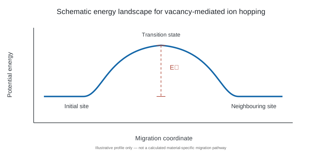
The jump frequency is often described using an Arrhenius-type expression:

\[ \Gamma=\nu_0\exp\left(-\frac{E_m}{k_{\mathrm B}T}\right) \]

where:

• \(\Gamma\) is the successful jump frequency;
• \(\nu_0\) is an attempt-frequency prefactor;
• \(E_m\) is the migration barrier;
• \(k_{\mathrm B}\) is Boltzmann’s constant;
• \(T\) is absolute temperature.

The attempt frequency is related to lattice vibrational timescales, but the effective prefactor can also include geometrical and entropic contributions. A real migration network may contain multiple inequivalent pathways and barriers.

Factors controlling the migration barrier

The migration barrier depends on more than the nominal ionic radius. Important factors include:

1. Bottleneck geometry along the migration pathway.
2. Local coordination and lattice distortion.
3. Electrostatic interactions between the migrating ion and surrounding cations.
4. Polarizability and flexibility of the anion framework.
5. Short-range defect interactions and local chemical disorder.
6. Changes in crystal symmetry or phase transitions with temperature.

A large oxygen-vacancy concentration does not guarantee high oxide-ion conductivity if the available migration pathways have high barriers or are poorly connected in three dimensions.

3. Vacancy concentration versus vacancy mobility

The conductivity of a material depends on both the number of mobile charge carriers and their mobility. For a single carrier species, a simple expression is

\[ \sigma=|z|e c\mu \]

where \(z\) is the carrier charge number, \(e\) is the elementary charge, \(c\) is the carrier number concentration and \(\mu\) is the mobility.

For oxygen vacancies, \(|z|=2\) in the common doubly ionized representation. This expression is useful conceptually, but the measured ionic conductivity is associated with the transport of the actual ionic species and may require correlation corrections.

The distinction between total and mobile vacancies is important. Some vacancies may be associated with dopants, trapped in defect complexes, ordered, or otherwise unavailable for long-range transport over the measurement timescale.

Why more dopant does not always mean higher conductivity

Acceptor doping can increase the oxygen-vacancy concentration. At low dopant concentrations, this can increase ionic conductivity. At higher concentrations, however, dopant–vacancy association, vacancy ordering, lattice distortion and changes in phase stability can reduce mobility.

Consequently, conductivity can exhibit a maximum as a function of dopant concentration. The optimum is material- and temperature-dependent; it should be measured rather than assumed.

4. Nernst–Einstein relation

For independent mobile charge carriers, the Nernst–Einstein relation connects conductivity to the diffusion coefficient:

\[ \sigma=\frac{c z^2 e^2 D}{k_{\mathrm B}T} \]

where \(D\) is the tracer diffusion coefficient under the ideal independent-carrier approximation.

For oxygen vacancies, this expression can be written using the vacancy concentration and vacancy charge. For oxide-ion transport, care is needed when translating vacancy diffusion into oxygen self-diffusion because the vacancy and oxygen-ion fluxes are related but opposite in direction.

In real solids, correlated jumps and collective motion can cause deviations from the ideal Nernst–Einstein prediction. A Haven ratio or related correlation factor is therefore used in some treatments to connect tracer diffusion and conductivity diffusion. The precise definition of the Haven ratio depends on the convention adopted; always state the definition when comparing values.

The relation is most useful as a framework for comparing transport measurements and atomistic calculations, not as a guarantee that measured conductivity can be predicted from a single diffusion coefficient without correction.

5. Arrhenius behaviour and activation energy

Ionic conductivity in many crystalline oxides follows an approximate Arrhenius relationship over a restricted temperature range:

\[ \sigma T=\sigma_0 \exp\left(-\frac{E_a}{k_{\mathrm B}T}\right) \]

Taking the natural logarithm gives

\[ \ln(\sigma T)=\ln\sigma_0 -\frac{E_a}{k_{\mathrm B}}\frac{1}{T} \]

A plot of \(\ln(\sigma T)\) against \(1/T\) is therefore expected to be linear when a single effective activation energy dominates.

If base-10 logarithms are used,

\[ \log_{10}(\sigma T)= \log_{10}\sigma_0 -\frac{E_a}{2.303k_{\mathrm B}}\frac{1}{T} \]

For a slope \(m\) obtained from a plot of \(\ln(\sigma T)\) versus \(1/T\),

\[ E_a=-m k_{\mathrm B} \]

If the horizontal axis is \(1000/T\), the slope must be multiplied by the corresponding factor of 1000 when converting to energy.

Migration energy is not always the measured activation energy

The measured activation energy can contain contributions from both defect formation and defect migration.

• In a doped oxide where the concentration of mobile defects is approximately fixed by extrinsic dopants, the activation energy may be dominated by migration and association effects.
• In an intrinsic regime, the equilibrium concentration of defects can be temperature-dependent, so defect formation contributes to the apparent activation energy.
• If defect association changes with temperature, the apparent activation energy can include dissociation contributions.
• If the dominant transport pathway changes, a single Arrhenius slope may not describe the full temperature range.

Therefore, do not automatically label every conductivity activation energy as the oxygen-vacancy migration barrier.

6. Bulk, grain-boundary and electrode contributions

A polycrystalline ceramic contains grains, grain boundaries, pores and electrode interfaces. These regions can have different defect concentrations, structures and transport properties.

In impedance spectroscopy, the measured response may contain contributions from:

• Bulk (grain interior): transport through the crystalline grains.
• Grain boundary: transport across interfaces separating adjacent grains.
• Electrode interface: charge transfer, surface exchange, gas conversion and contact effects.

These contributions can sometimes be separated by their characteristic capacitances and relaxation frequencies. They are not guaranteed to appear as three clean semicircles.

Brick-layer model

A simplified brick-layer model treats grains as conducting blocks separated by thin grain-boundary layers. For current passing through a series stack of grain and grain-boundary regions, the total resistance is

\[ R_{\mathrm{total}}=R_{\mathrm{bulk}}+R_{\mathrm{gb}} \]

For a homogeneous region of thickness \(L_i\), cross-sectional area \(A\) and conductivity \(\sigma_i\),

\[ R_i=\frac{L_i}{\sigma_i A} \]

The corresponding conductivity is

\[ \sigma_i=\frac{L_i}{R_i A} \]

The effective length assigned to a grain-boundary contribution requires a model. In a brick-layer approximation, the grain-boundary thickness and number of boundaries crossed must be considered before converting a measured resistance into an intrinsic grain-boundary conductivity.

A large grain-boundary resistance can dominate the total resistance even when the grain interiors are highly conductive.

Space-charge effects

Grain boundaries can exhibit defect segregation and electrostatic potential gradients. A charged grain-boundary core may create adjacent space-charge regions in which mobile vacancies or other defects are depleted or accumulated.

For example, oxygen-vacancy depletion near a positively charged boundary can suppress oxide-ion transport across that region. The effect depends on the boundary chemistry, dopant distribution, atmosphere and defect model. It is not correct to assume that every grain boundary is intrinsically blocking or that every disordered boundary is a fast diffusion path.

7. Grain size and processing effects

Grain size changes the fraction of material occupied by grain boundaries. If grain boundaries are more resistive than grain interiors, reducing grain size can increase the total grain-boundary contribution.

This is one reason why two ceramics with the same nominal composition can show different conductivities after different sintering schedules.

Important processing variables include:

• Calcination and milling history;
• Powder particle-size distribution and agglomeration;
• Green density and forming pressure;
• Sintering temperature and dwell time;
• Heating and cooling rates;
• Atmosphere and oxygen partial pressure;
• Impurity segregation and secondary-phase formation.

A higher sintering temperature may increase density and reduce porosity, improving measured conductivity. At the same time, grain growth, dopant redistribution, volatilization or secondary-phase formation may alter transport. The net effect is not universal.

Separating porosity from intrinsic transport

Porosity reduces the effective cross-sectional area available for conduction and can increase tortuosity. A porous ceramic can therefore show a lower apparent conductivity even if the intrinsic conductivity of the solid phase is unchanged.

Report relative density and, where possible, microstructural information alongside conductivity. Avoid comparing conductivity values from ceramics with substantially different porosity without considering the geometric effect.

8. Extracting conductivity from impedance measurements

For a parallel-plate geometry, conductivity is calculated from resistance using

\[ \sigma=\frac{L}{RA} \]

where \(L\) is the distance between electrodes and \(A\) is the electrode area. Use consistent SI units to obtain conductivity in S m\(^{-1}\).

For a cylindrical pellet with diameter \(d\),

\[ A=\frac{\pi d^2}{4} \]

and therefore

\[ \sigma=\frac{4L}{R\pi d^2} \]

The resistance must be assigned to the relevant contribution. If the objective is bulk conductivity, use the bulk resistance rather than the total resistance when the bulk and grain-boundary processes can be reliably separated.

Practical impedance workflow

1. Measure pellet thickness and electrode area carefully.
2. Confirm electrode coverage, contact quality and sample sealing.
3. Stabilize the sample at the target temperature and atmosphere.
4. Select a frequency range broad enough to capture the relevant relaxations.
5. Use a perturbation amplitude within the linear-response regime.
6. Check for inductive artefacts, open-circuit drift and unstable contacts.
7. Fit with physically defensible equivalent circuits or use complementary analysis such as DRT.
8. Validate fitted parameters against capacitance scale, temperature dependence and repeatability.
9. Convert each assigned resistance to conductivity using the correct geometry.
10. Report whether the value is bulk, grain-boundary, total ionic or total electrical conductivity.

An equivalent-circuit fit is not proof of a unique physical mechanism. The assignment of a response to a grain, grain boundary or electrode process should be supported by its capacitance, frequency range, temperature dependence and independent evidence.

9. Ionic versus electronic conductivity

A solid electrolyte should conduct the target ion while suppressing electronic leakage. The total conductivity can be expressed as

\[ \sigma_{\mathrm{total}}= \sigma_{\mathrm{ion}}+ \sigma_{\mathrm{e}}+ \sigma_{\mathrm{h}} \]

where the terms represent ionic, electron and hole contributions.

The ionic transference number is

\[ t_{\mathrm{ion}}= \frac{\sigma_{\mathrm{ion}}} {\sigma_{\mathrm{total}}} \]

For an ideal ionic electrolyte, \(t_{\mathrm{ion}}\) approaches unity under the specified operating conditions. The transference number can vary with temperature, oxygen partial pressure and water-vapour pressure.

A high total conductivity does not necessarily indicate a good electrolyte. If electronic conductivity is significant, internal electronic current can reduce the electrochemical efficiency of a cell or pump.

Possible approaches to distinguish ionic and electronic contributions include blocking-electrode measurements, Hebb–Wagner polarization, oxygen concentration-cell measurements and controlled-atmosphere conductivity measurements. Each method has assumptions and experimental limitations.

10. Oxide-ion and proton transport are not identical

Oxide-ion conduction is commonly described by oxygen-ion jumps between lattice oxygen sites and vacancies. Proton conduction in hydrated oxides is often described by proton transfer between neighbouring oxygen ions, coupled to reorientation of hydroxyl groups.

The two mechanisms respond differently to temperature, hydration and lattice geometry. In proton-conducting perovskites, water incorporation creates hydroxyl defects, while dehydration at higher temperature can reduce the proton concentration.

For this reason, conductivity measurements in humid and dry atmospheres should not be compared as if only the migration mobility had changed. The carrier concentration may also be different.

11. Worked calculation: conductivity of a ceramic pellet

Consider a ceramic pellet with:

• Thickness \(L=1.20\ \mathrm{mm}=1.20\times10^{-3}\ \mathrm{m}\);
• Diameter \(d=10.0\ \mathrm{mm}=1.00\times10^{-2}\ \mathrm{m}\);
• Assigned resistance \(R=250\ \Omega\).

The electrode area is

\[ A=\frac{\pi(1.00\times10^{-2})^2}{4} =7.854\times10^{-5}\ \mathrm{m^2} \]

The conductivity is

\[ \sigma= \frac{1.20\times10^{-3}} {250\times7.854\times10^{-5}} \]

\[ \boxed{\sigma=0.0611\ \mathrm{S\,m^{-1}}} \]

Converting to S cm\(^{-1}\),

\[ \boxed{\sigma=6.11\times10^{-4}\ \mathrm{S\,cm^{-1}}} \]

This result is only as meaningful as the resistance assignment and sample geometry. If 250 \(\Omega\) is the total resistance of bulk and grain-boundary processes, the calculated value is an effective total conductivity, not the intrinsic bulk conductivity.

12. Common interpretation errors

• Using the total impedance resistance as bulk resistance: bulk and grain-boundary contributions may be distinct.
• Ignoring sample geometry: conductivity depends on thickness and electrode area.
• Calling the apparent activation energy a migration barrier: defect formation and association may contribute.
• Assuming more vacancies always improve conductivity: mobility and defect association matter.
• Ignoring porosity: the measured conductivity is affected by the effective conducting cross-section.
• Treating every high-frequency arc as bulk without checking capacitance: frequency alone is insufficient.
• Equating a DRT peak with one unique process: peak assignments require independent validation.
• Comparing dry and humid measurements without considering carrier concentration: hydration changes the defect population.
• Ignoring electronic leakage: total conductivity can overstate useful ionic transport.
• Reporting conductivity without atmosphere and temperature: the value is not reproducible or interpretable.

13. Minimum reporting checklist

For a publishable ionic-transport study, report:

1. Exact composition, dopant concentration and phase purity.
2. Synthesis, calcination, pressing and sintering conditions.
3. Relative density, grain size and relevant microstructural observations.
4. Pellet dimensions, electrode material and electrode area.
5. Measurement temperature, atmosphere, oxygen partial pressure and humidity.
6. Frequency range, AC amplitude and equilibration protocol.
7. Equivalent circuit or other analysis method and fit quality.
8. Resistance assignment and geometry used for each conductivity.
9. Arrhenius plot, fitting interval, equation and activation-energy uncertainty.
10. Evidence supporting ionic versus electronic transport.
11. Repeatability and uncertainty from sample dimensions and resistance fitting.

Further reading

• J. B. Goodenough, “Oxide-Ion Electrolytes,” Annual Review of Materials Research 33 (2003), 91–128. https://doi.org/10.1146/annurev.matsci.33.022802.091651.
• L. Malavasi, C. A. J. Fisher and M. S. Islam, “Oxide-ion and proton conducting electrolyte materials for clean energy applications: structural and mechanistic features,” Chemical Society Reviews 39 (2010), 4370–4387. https://doi.org/10.1039/B915141A.
• P. Knauth, “Solid-State Ionics: Roots, Status, and Future Prospects,” Journal of the American Ceramic Society 85 (2002), 1654–1680. https://doi.org/10.1111/j.1151-2916.2002.tb00334.x.
• G. Gregori, R. Merkle and J. Maier, “Ion conduction and redistribution at grain boundaries in oxide systems,” Progress in Materials Science 89 (2017), 252–305. https://doi.org/10.1016/j.pmatsci.2017.04.009.
• R. A. De Souza, “Ion Transport in Metal Oxides,” in Resistive Switching, Wiley (2016). https://doi.org/10.1002/9783527680870.ch5.

Related articles

• Defect equilibria in functional oxides
• Oxygen vacancies and defect chemistry in functional oxides
• Measuring oxygen nonstoichiometry in functional oxides
• Electrochemical impedance spectroscopy: a practical guide
• Impedance data analysis: equivalent circuits and DRT
• Proton-conducting oxides

Conductivity values should always be reported with temperature, atmosphere, sample geometry and a clear definition of the resistance used in the calculation. A fitted impedance component is a model assignment that requires physical validation.